Home >
Models

Mathematical formulations for ASONIKA

1 MODELS OF THE THERMAL PROCESSES (ASONIKA-T and ASONIKA-TM)

2 MODELS OF THE MECHANICAL PROCESSES (ASONIKA-TM)

2.1 Models of the mechanical processes based on the finite difference method

2.2 Models with harmonic vibrations

2.3 Models with random vibrations, impact, and linear acceleration

2.4 Models with acoustic noise

3 RELIABILITY MODELS (ASONIKA-B)

1 MODELS OF THE THERMAL PROCESSES (ASONIKA-T and ASONIKA-TM)

By exploiting the electro-thermal analogy (ETA), the thermal processes occurring in the electronic assemblies can be represented in the form of an equivalent electric circuit. This circuit can then be analyzed by means of the well-developed numerical techniques for electric circuits. Mathematically, it is done by replacing the partial differential equations with the finite-difference equations. Consider the following steady-state Fourier-Kirchhoff differential equation describing the heat transfer in a solid isotropic body

, (1.1)

where λ – thermal conductivity, q_V – power density of the internal energy sources, Т – temperature, - Laplacian operator.

Assuming that continuous processes can be replaced with discrete processes, equation (1.1) can be written in the finite-difference form as follows

(1.2)

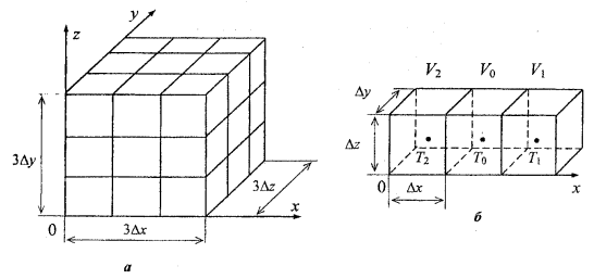
Figure 1.1 Discretization of a solid body into elementary volumes (а), and a set of such volumes along the x-axis (б).

Figure 1.1a shows a solid body discretized into elementary volumes of dimensions Δx, Δy, Δz. Consider a set of elementary volumes along the x-axis consisting of the volume V₀ and the two adjacent volumes V₁, V₂, as shown in figure 1.1б. Denote the temperatures at the center of each volume Т₀, Т₁, Т₂ (assume that the volumes are isothermal).

Volume V₀ contains internal energy sources with the power density q₀.

Then, for the volume V₀, the x component of the Laplacian in (1.2) can be written as (using the forward difference):

(1.3)

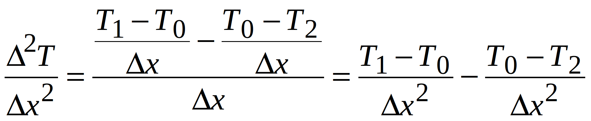
Similarly, considering the elementary volumes along y- and z-axis (figure 1.2), the remaining y and z components of the Laplacian in (1.2) are:

Figure 1.2 Two sets of the elementary volumes along the y- and z-axes.

(1.4)

(1.5)

Using (1.3), (1.4) and (1.5), equation (1.2) becomes:

(1.6)

Multiplying both sides of (1.6) by the volume V₀= Δx · Δy · Δz, we get

(1.7)

where Q₀=q₀ ·Δx · Δy · Δz – thermal power dissipated in the volume V₀.

Define:

, ,

These quantities have the units of (W/K) and represent thermal conductances between adjacent volumes in the x-, y-, and z-directions, respectively. Thus, equation (1.7) becomes:

(1.8)

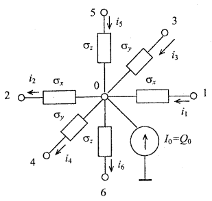
Figure 1.3 Equivalent electrical circuit representing the steady-state heat transfer in the elementary volume V₀.

The finite-difference equation (1.8) describes heat transfer in the elementary volume V₀. Figure 1.3 shows the electric circuit analog of equation (1.8) based on the Kirchhoff’s first law for the sum of currents at the 0-th node.

Boundary conditions

Let’s consider now a boundary volume along x-axis (volume V₁ in figure 1.4). As can be seen in the figure, this elementary volume is located outside the solid body; it is located in the environment surrounding the body. Step Δх outside the solid body is introduced artificially.

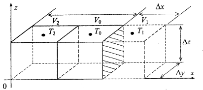
Figure 1.4 Boundary elementary volume V₁.

Equation (1.6) for the boundary volume V₁has the following form:

(1.9)

where λ_Г is not the thermal conductivity of the isotropic body but the conductivity of the interval which includes the boundary between the body and the surrounding medium.

In the experimental analysis of the heat-conducting properties of an interface, when trying to determine the law of heat-exchange between the surface of the body and the environment, the quantity known as the heat transfer coefficient is determined, α = λ_Г/Δх. Various boundary conditions can be specified at the body-environment interface.

The boundary condition of the first kind specifies the temperature of the surface (Т_п) as a function of position and time:

Т_п=f(x_п, y_п, z_п, τ) (1.10)

where x_п, y_п, z_п - coordinates, τ - time (for steady-state τ is excluded).

The boundary conditions of the first kind cannot be specified during the design stage because the design is not yet implemented and the temperatures of the boundary surfaces are not yet experimentally determined.

The boundary condition of the second kind specifies the density of the heat flow through the surface as a function of position and time:

q_п=f(x_п, y_п, z_п, τ) (1.11)

Such boundary conditions occur on the boundaries between the components of the electronic assembly and the surrounding air.

The heat flux density q_п can be described by the Newton’s law of cooling with the heat transfer coefficient α:

q_п= α · (Т_п – Т_ср)

If equation (1.9) is manipulated the same way as equation (1.6), we obtain

, (1.12)

where G^’_x= α · Δy · Δz - thermal conductance of the surface in contact with the surrounding medium.

Figure 1.5 shows the electric circuit analog of equation (1.5) based on the Kirchhoff’s first law for the sum of currents at a node (in the figure, node 1 represent surface of the body).

Figure 1.5 Equivalent electrical circuit representing the heat transfer in the boundary elementary volume with the specified boundary conditions of the second kind.

The boundary condition of the third kind specifies the ambient temperature and the law of heat-exchange between the surface of the body and the environment. Such boundary conditions occur on the boundaries between the surface of the elements and the surrounding medium. For the boundary condition of the third kind, equation (1.12) has the following form:

(1.13)

The difference between (1.13) and (1.12) is that the temperature Т₁ is known and equal to Т_ср. Figure 1.6 shows the electric circuit analog of equation (1.13) based on the Kirchhoff’s first law for the sum of currents at a node.

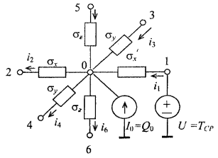
Figure 1.6 - Equivalent electrical circuit representing the heat transfer in the boundary elementary volume with the specified boundary condition of the third kind.

Boundary condition of the fourth kind specifies the temperature or its gradient at the boundary between the two media. Such boundary conditions occur on the boundaries between two media with different conductivities. For example, the boundary between a semiconductor component and a heat sink, transformer and packaging, two connected components of the assembly, etc.

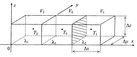
Figure 1.7 Boundary between of two solid bodies with different conductivities.

Consider the boundary between two solid bodies with different conductivities (figure 1.7). Equation (1.6) for such a boundary element has the following form:

(1.14)

where λ₀_Г₁is the conductivity of the interval which includes the body with conductivity λ₁, body with conductivity λ₂, and the boundary between them.

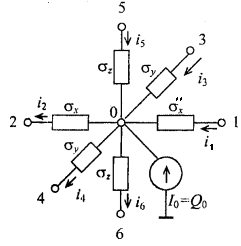
Figure 1.8 - Equivalent electrical circuit representing the heat transfer in the elementary volume located at the boundary between two solid bodies where the boundary conditions of the fourth kind is specified.

If equation (1.14) is manipulated the same way as equation (1.6), we obtain

, (1.15)

where - thermal conductance between two solid bodies.

Figure 1.8 shows the electric circuit analog of equation (1.15) based on the Kirchhoff’s first law for the sum of currents at a node.

If the thermal contact between two solid bodies is assumed to be perfect, the temperatures of the boundary volumes is taken to be equal, i.e. Т₁=Т₀.

Equation (1.15) becomes:

(1.16)

Figure 1.9 showstheelectriccircuitanalogofequation (1.16) basedontheKirchhoff’sfirstlawforthesumofcurrentsatanode.

Figure 1.9 - Equivalent electrical circuit representing the heat transfer in the elementary volume located at the boundary between two solid bodies with perfect thermal contact.

Thus, the heat transfer in a solid body with boundary conditions of any kind can be modeled by the equivalent electrical circuit.

Using these elementary heat transfer models with appropriate specified boundary conditions, the electro-thermal analogy can be extended to model thermal processes in the electronic assembly. The models of thermal processes (MTP) are based on the following analogies: voltage at a node of an equivalent electric circuit is equivalent to the temperature at that node, electric conductivity - thermal conductivity, electric current – thermal flow, current source directed into the node – heat capacity rate, current source directed out of the node – heat absorption capacity, voltage source – specified temperature of the corresponding part of the electronic assembly.

Following this approach, the electronic assembly is subdivided into volumes which are small enough to be considered isothermal. Representation of the assembly by a set of thermal conductances between such volumes, results in a large scale equivalent electric circuit. This circuit can be analyzed on a computer using the methods of electric circuit analysis.

When solving non-steady-state problems, the equivalent electric circuits will also include capacitors which represent thermal capacities of the corresponding elementary volumes. Equation (1.1) for the non-steady-state heat transfer has the following form (the last term explains the presence of capacitors):

(1.17)

where С_р – specific heat capacity, J/(kg·К); ρ – material density kg/m³.

After the manipulations similar to (1-6) – (1.8), we can obtain:

(1.18)

where С₀ – heat capacity of volume V₀.

Figure 1.10 shows the electric circuit analog of equation (1.18)

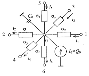
Figure 1.10 - Equivalent electrical circuit representing the non-steady-state heat transfer in the elementary volume V₀.

In the non-steady-state heat transfer analysis, initial conditions should be specified in addition to the boundary conditions. Initial condition specifies the temperature distribution at the initial time τ₀

Т=f(x, y, z, τ)

This function is defined for some time interval Δτ, during which the thermal processes are being analyzed. To facilitate the analysis of the thermal processes in the electronic assemblies, it is convenient toforma topologicalrepresentationof thermal models.

Topological model is a model represented in the form of an undirected graph. In the MTP, vertices (nodes) of such a graph represent structural elements and components of the electronic assembly (heated zones). Branches (edges) represent thermal flow. Nodal variables are computed temperatures (Т_i), variables of the branches – heat flux (Ψ_ij), and parameters of the branches – thermal conductance (Х_ij). In general, two types of branches can be identified in the non-steady-state heat flow analysis: 1-st type – dissipative branches where the values or analytical expressions of the thermal conductance (X_ij) are known; 2-nd type – conservative branches where the values or analytical expressions of the heat capacity (C_ij) are known.

Unlike in other models, in topological thermal models boundary conditions of any kind and combination can be easily specified with the help of the corresponding components of the graph (branches, specified temperature sources and/or sources with specified thermal power). Other advantages of the topological model are: relatively simple transition to other mathematical models; the ability to use general methods for formulating and solving mathematical models, including the theory of sensitivity.

A topological model of the thermal processes (MTP) in an element can be divided into two parts:

1. Parts which describe thermal processes in the element without taking cooling into account (boundary conditions).

2. Parts which take cooling into account.

Parts of the MTP of the first type represent thermal models of the structural components (printed electronic parts, function cells, electronic parts without packaging). These models can be easily obtained by using the finite-difference approximations of the heat transfer equation. It should be noted that such approach makes it possible to form parts of the MTP with different level of detail. Such parts can be used in different stages of the design, using hierarchical approach. When analytical model are used, computation of the parameters of the MTP is based on the geometrical and thermo-physical parameters of the structure; therefore, any feature of the structure can be taken in to account.

Parts of the MTP of the second type represent boundary conditions of the 1-4 kind and their combinations. They are expressed through geometrical and thermo-physical parameters of the structure and thermo-physical parameters of the surrounding environment.

Among various thermal processes occurring in the elements, simple forms of heat-exchange can be identified and used to construct topological models of the thermal processes (MTP). For clarity of representation, graphic images of the topological branches can be introduced with original designations assigned to the components of the graphs.

2 MODELS OF THE MECHANICAL PROCESSES (ASONIKA-TM)

2.1 Models of the mechanical processes based on the finite difference method

There are many ways to assemble various electronic components. Some assemblies, however, can be identified as less efficient at protecting the terminals of the components against mechanical vibrations. Although any mechanical effect can cause time-varying loadings in the terminals, fatigue-failure is mainly caused by the long-term cyclic loadings such as harmonic and random vibrations, and acoustic noise. Comparing to these loadings, short-term loadings such as impact and linear acceleration do not contribute much to the fatigue accumulation. Therefore, it is necessary to develop models of the components subjected to vibrations and noise.

To determine dynamic characteristics of an electronic assembly two problems have to be solved: the first one determines natural frequencies and forms of vibrations of the structure, and the second determines the amplitudes of the forced oscillations of the components at different locations in the assembly under specified external vibration (load). It is then possible to determine mechanical loadings and strength tolerances of the structure and assess the probability of non-failure under vibration.

In practice, the applicability of the analytical methods for solving such problems is very limited. Modern electronic assemblies represent complex mechanical systems with numerous elastic and rigid connections. In addition, various elements of such a system are often joined together in a fashion that is not standard for structural mechanics. Moreover, elements of the assembly are often mechanical structures themselves, which can resonate and, therefore, significantly increase mechanical loadings. It is difficult to create an analytical model which is simple and, at the same time, sufficiently accurate to represent physical and dynamic properties of such a mechanical system. A number of mathematical difficulties usually arise when trying to establish and solve the equations of motion of such a structure.

Therefore, dynamic properties of the electronic assemblies are usually on a computer using numerical methods. The Finite Element Method is one of the most effective methods for solving problems which involve complex practical structures. Over the years it became one of the most popular and wide-spread techniques. Nowadays, there exist many software packages based on the Finite Element Method. Among them, ANSYS is one of the most versatile. Advanced programming algorithms of this package allow significant automation of the process of the component design and their discretization into finite elements.

The analysis of vibrations in electronic circuit boards is often based on the Kirchhoff–Love theory of plates. The assumption made in this theory is the following: all straight lines normal to the mid-surface of the plate remain straight and normal to the mid-surface after deformation. Thus, the coordinate along the thickness of the plate can be excluded from the model.

The form of the equation describing forced oscillations in a printed board assembly (PBA) depends on the accepted hypothesis about the internal damping force. If these force is assumed to be proportional to the deformation, then the equation of motion is

(2.1)

where - vertical displacement (bending) of the printed circuit board at the point with coordinates x, y and time t; - mass of the PCB per unit area ; - cylindrical stiffness long x- and y-axis, respectively; - stiffness; - complex rotational stiffness; - complex shear modulus; h – thickness of the PCB; ,, - complex modulus of elasticity along x and y directions and at an angle of 45⁰, where

where i=1,2,45; - logarithmic decrement of damping; - Poisson coefficients of the material along x and y directions and at an angle of 45, respectively (x and y axis coincide with the sides of the PCB); - external force per unit area causing oscillations.

To use this equation for modeling mechanical processes in a PBA subjected to vibrations, impacts, linear accelerations and acoustic noise, the following two criteria should be satisfied.

The first criterion (Petrashen criterion) is:

where - angular frequency of oscillations; - material density.

Let’s substituting the values of for the printed circuit board made of the epoxy glass laminate sheet. The values which maximize the left-hand side are: . Then, the left-hand side is equal to 0.013<<1.

The second criterion (Ross criterion) is:

Using the same values for , and , , the left-hand side is equal to .

Thus, equation(2.1) can be used to model themechanical processes in the PBA for all types ofmechanical effects,whose spectrumlies within2000 Hz. The following sections present models based on (2.1) which describe PBAs subjected to harmonic and random vibrations, impact, linear acceleration and acoustic noise. Both, analytical and finite-difference models will be considered. The former are used for the assemblies with uniform arrangement of the components whereas the latter are used for the arbitrary arrangement.

2.2 Models with harmonic vibrations

Let’s employ the finite-difference method to solve equation (2.1). To transform (2.1) to the frequency domain, assume that the unknown variable, vertical displacement (bending) of the PCB at a point i with coordinates (x,y) and time t, can be written as:

(2.2)

where _i – amplitude of the vertical displacement at point i.

Figure 2.1 shows sketch of a PBA with the superimposed uniform rectangular grid. The step size of the grid along x and y directions can be different. Figure 2.2 shows numbering of the nodes surrounding some node i.

For better accuracy, the special derivatives will be approximated using central difference. Thus, the partial derivatives in (2.1) can be replaced with the following approximate finite-difference expressions:

(2.3)

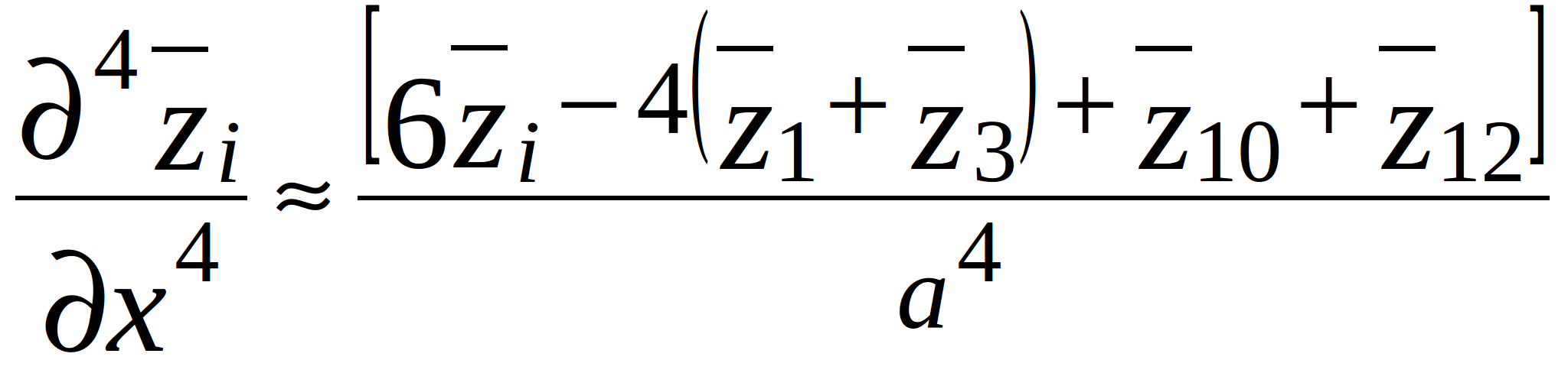
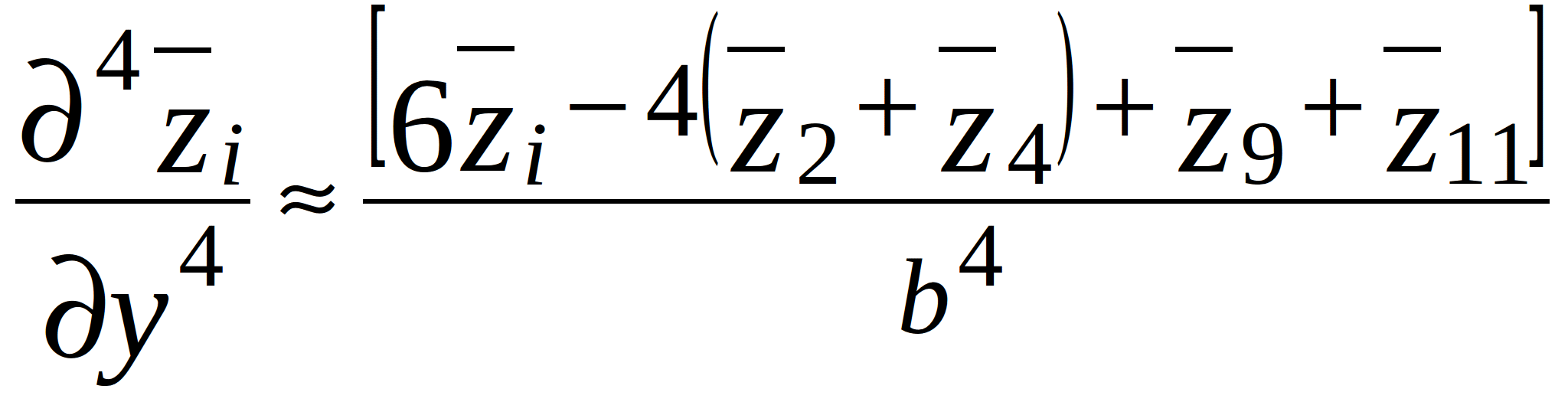
where a and b – step-size along x- and y-axis as shown in figure 2.1; - vertical displacements of the PCB from the equilibrium at the points 1,…,12, located around node i as shown in figure 2.2.

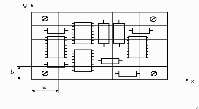
Figure 2.1 Sketch of a printed circuit board with superimposed grid.

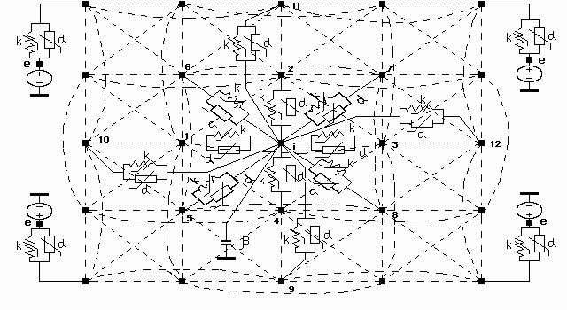
Figure 2.2 Topological model of a PCB subjected to harmonic vibration.

The model also takes into account temperature.

In general, external force per unit area causing oscillations at any point i and time t can be written as:

(2.4)

Substitute (2.2) - (2.4) in (2.1). After grouping terms with the same displacement, we get:

(2.5)

where - mass of the i-th node per unit area.

Since the grid in figure 2.1 is uniform, the area of each rectangle is . Therefore, after multiplying (2.5) by ab, the mass per unit area in the last term becomes the mass of such a rectangle. Divide (2.5) by , substitute the following expression for stiffness

and separate conservative and dissipative parameters. After these manipulations, (2.1) can be written in generalized notation:

(2.6)

where - nodal variables in the topological model of the PCB ( - nodes where PCB supports are connected to the base);

(2.7)

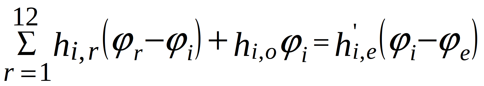
conductance of the branches in the topological model. Note that for the internal nodes (located more than two nodes away from the edges):

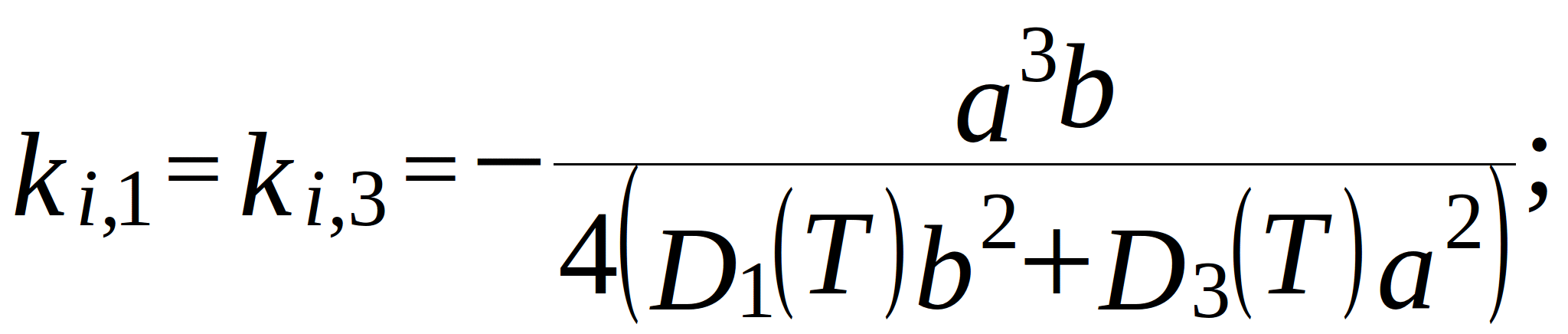
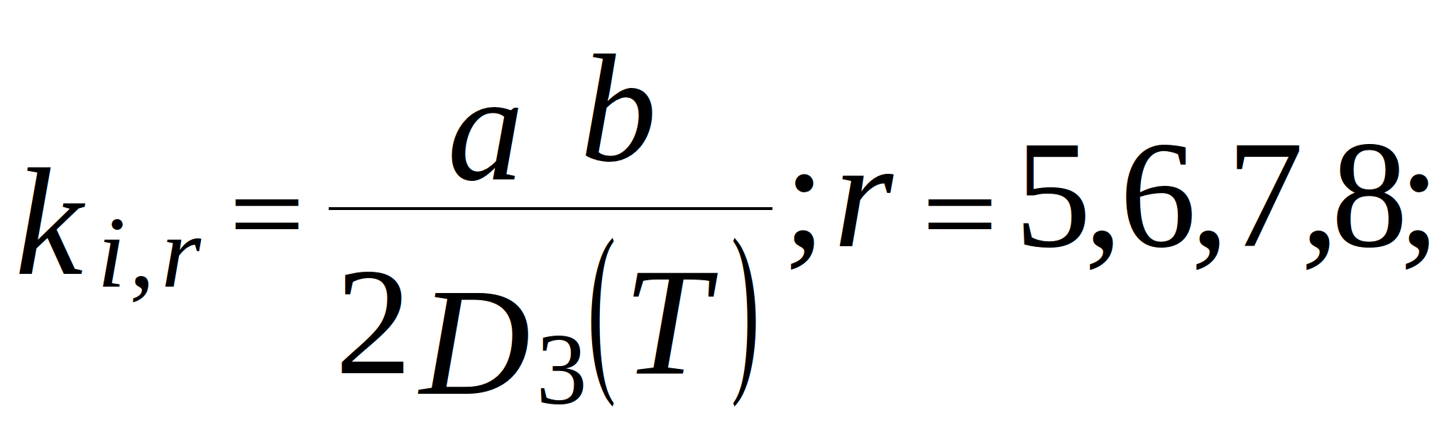
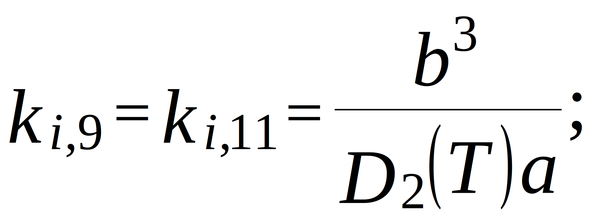
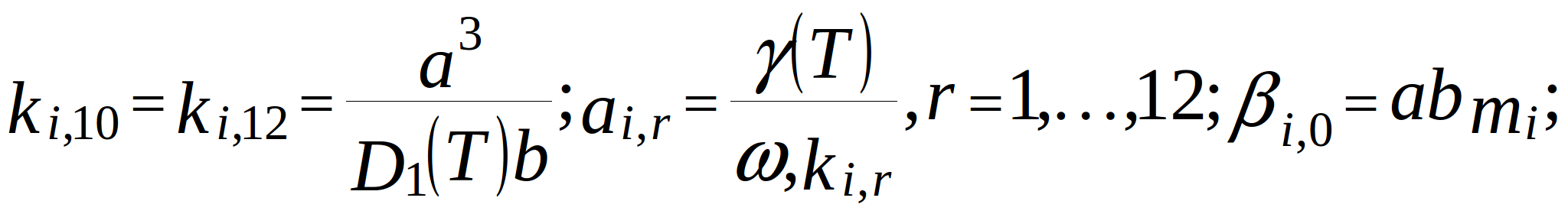
where and - grid steps along x- and y-axis; - mechanical loss coefficient of the support material (constant, because support usually oscillates at frequencies far from resonance); - rigidity of the PCB supports under tension. In this model, the temperature is taken into account thorough the temperature-dependent parameters - modulus of elasticity (cylindrical stiffness) and mechanical loss coefficient. In the topological mechanical model of the PCB, these dependences are represented by adjustable elements - resistors and inductors.

For the nodes which are located on the edge, one node away from the edge, at the corner, and one node away from the corner, the branch conductances are:

Node i is on the edge:

Nodei is one node away from the edge:

Node i is on the edge and one node away from the corner:

Nodei is not on the edge but one node away from the corner:

Node i is at the corner:

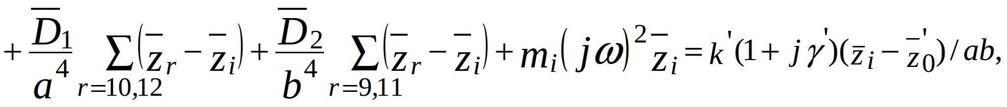
As can be seen from (2.6), any -th node in the topological model should be connected to 12 surrounding nodes (see figure 2.2) and one common node (ground) with zero potential (in figure 2.2 this node is denoted as a solid thick line). Dashed lines in figure 2.2 represent branches in the topological model. Moreover, if the i-the node represents the PCB support, it should be connected to the e-th node. Figure 2.2 also shows electrical equivalent representation of the conservative () and dissipative () components. Each i-th node is connected to the common node by a branch with conservative parameter . The right-hand side of equation (2.6) is zero for all nodes except the onces which are connected to the e-th node, that is PCB support.

The mass and cylindrical stiffness of the discrete elements are taken into account the same way as in analytical model

The finite difference expressions for stiffness at the internal i-th node are:

(2.8)

(2.9)

2.3 Models with random vibrations, impact, and linear acceleration

When the arrangement of the components on the PCB is non-uniform, the analysis of the mechanical processes due to random vibrations can be performed using Monte-Carlo method. Let’s solve equation (2.1) in the time domain using the finite-difference method. The partial derivative in time can be written in the finite-difference form as follows:

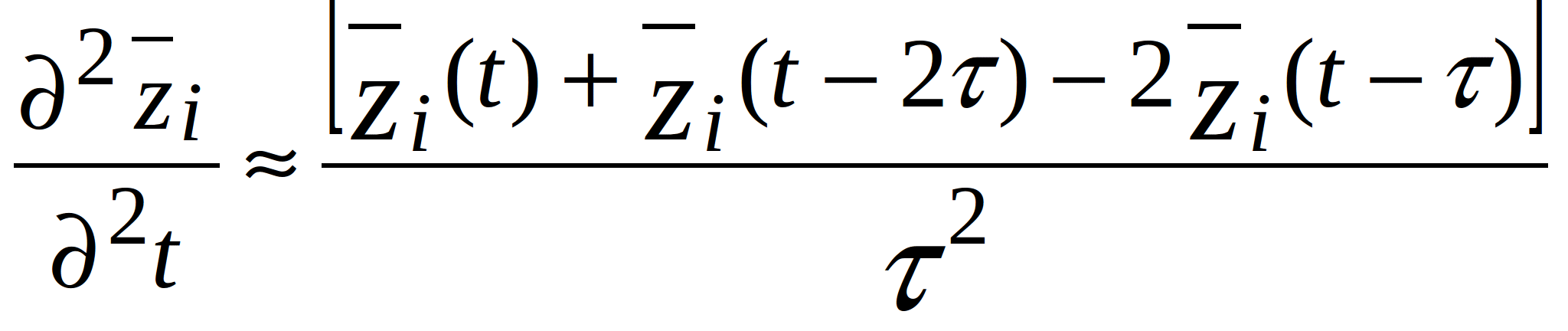(2.10)

where - discretization step in time; - total time during which the random process is active; - number of discretization points.

The partial derivatives in space are replaced with the corresponding approximate expressions. Taking into account the discretization in time, let’s introduce two additional point to the already existing thirteen and, thus, get a 15-point scheme. Then, expression (2.10) becomes:

(2.11)

In general, arbitrary time-dependent external force per unit area exciting the oscillations at any point i on the PCB, can be written as

(2.12)

where - instantaneous vibration displacement of the base.

Since vibration acceleration is usually specified, vibration displacement is found by integrating the acceleration twice. This integration is done numerically because the acceleration can be a very complex function of time.

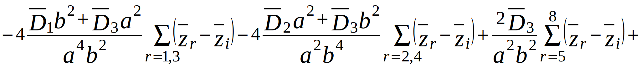
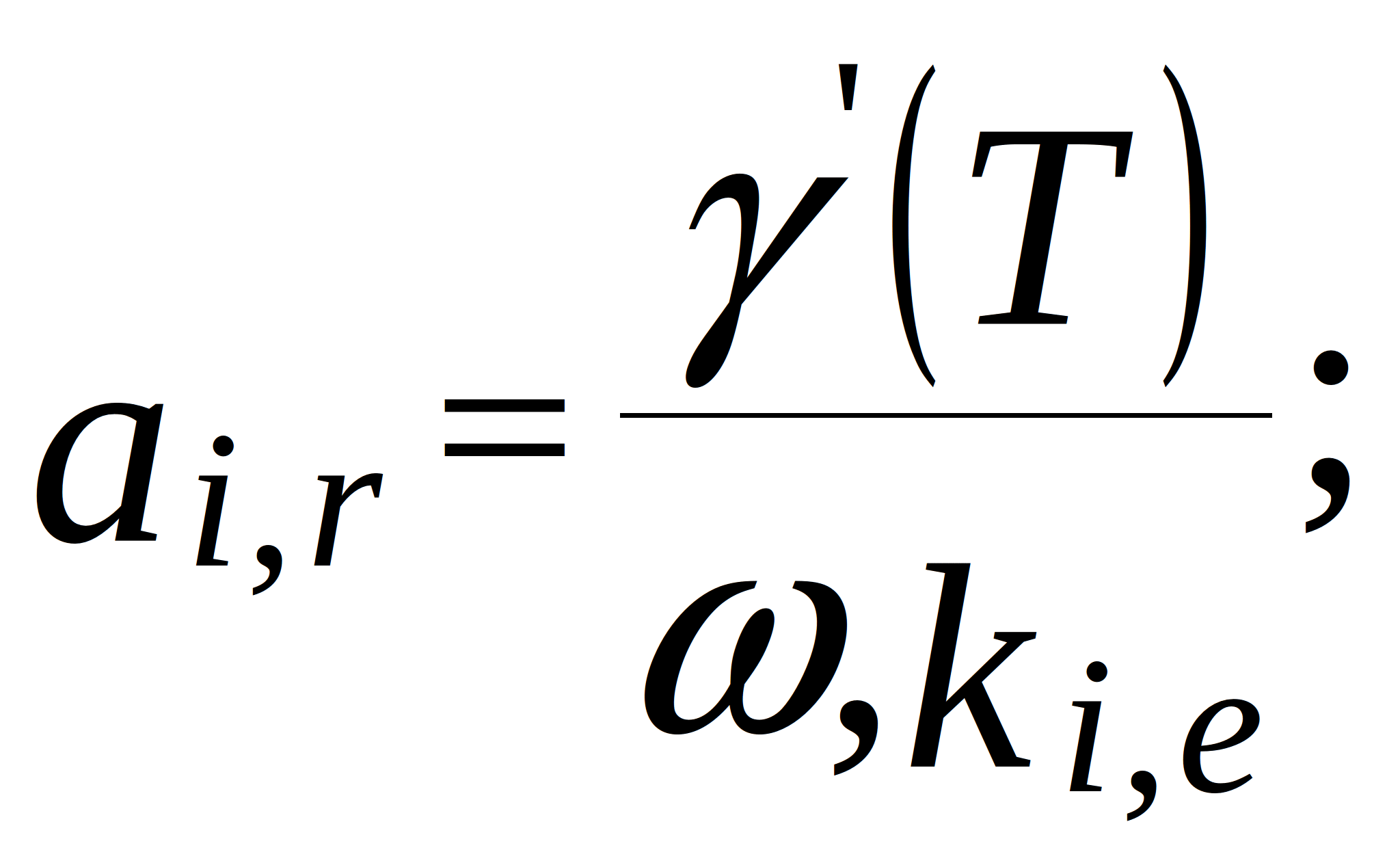
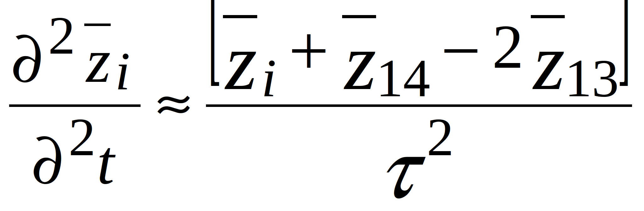
After replace the partial derivatives in (2.1) with the corresponding finite-difference expressions, substituting (2.11) and (2.12), and grouping terms with the same displacement, (2.1) can be written in generalized notation:

(2.13)

where , , , , - nodal variables in the topological model of the PCB; , - vertical displacement (bending) of the PCB at the i-th and r-th nodes at time t; - displacement of the supports at time t;

- mass of the i-th node per unit area.

Expression (2.13) contains artificially introduced frequency . In the topological model, it represents frequency of the alternating current in the circuit.

The time domain topological model of the PCB, which includes temperature, is almost identical to the model with harmonic vibration shown in figure 2.2. The difference is the addition of the branches (see figure 2.3) from nodes 13 and 14 and the exclusion of the branches connecting each i-th node to the common node. As a result, in the time domain models there exist 3 time layers; whereas, model in the frequency domain are discretized only in space coordinates. In addition, the parameters and , as can be seen in figure 2.3, are independent of temperature.

During the simulations, displacement is determined. The acceleration is found by taking the second time derivative of displacement. This differentiation is done numerically because the displacement can be a very complex function of time.

Vibrations with multiple harmonics, impact and linear acceleration can be defined as a single instance of the random process. Therefore, models of the PCBs subjected to these loadings can be realized as the model of the PCB under random vibration based on the finite-difference method and described by expression (2.13).

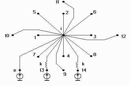
Figure 2.3 Topological model of the printed circuit board subjected to random vibration. The model also takes into account temperature.

2.4 Models with acoustic noise

Acoustic noise is a stationary random process like “white noise”. Therefore, the model with random vibrations can also be used to model acoustic noise in the range up to 2000 Hz. Severalmodifications, however, arenecessary. The difference between the loading due to the acoustic noise and the loading due to the mechanical vibration is in the distributed nature of the force which depends not only on the intensity of the sound but also on the area of the device. Mechanical vibrations are mainly transferred to the device through the supports of the structure. Thus, taking into account the distributed nature of the acoustic noise loading, acoustic pressure can be written as:

(2.14)

where - uncorrelated normally distributed random variable whose variance defines the spectrum of the random function and the standard deviation is the specified acoustic pressure.

Since acoustic noise creates distributed loading on the surface of the PCB, expression (2.13) will be slightly different for the discrete model. The external force per unit area causing the oscillations can be written as:

(2.15)

At the points anchorage there also exist elastic force and friction . Then, according to the D’Alembert’s principle, the force per unit area at the points anchorage is

Elastic force and friction can also be expressed similarly to (2.12)

where - absolute displacement due to the oscillation of the supporting structure (block). Then

(2.16)

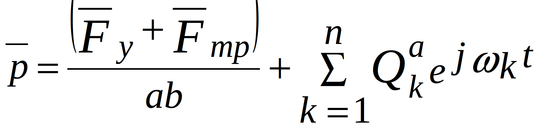
After substituting these expressions in (2.1) and grouping term with the same displacement, equation (2.1) for the i-th node can be written (in time domain) in generalized notation:

(2.17)

where 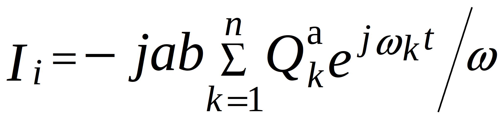- source current. If the node is not connected to the support, .

Thus, unlike in model (2.13), each i-th node is connected to the common node by a branch with the current source which has internal impedance (see figure 2.4а). For the nodes connected to the PCB support, the topological model is shown in figure 2.4б.

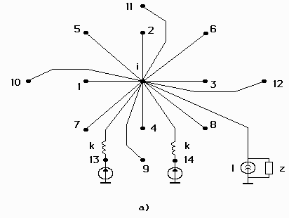
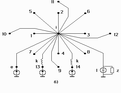
Figure 2.4 Topological model of the printed circuit board subjected to acoustic noise. The model also takes into account temperature.

a – node without support; б – node with support

3 RELIABILITY MODELS (ASONIKA-B)

The probability of no failure (reliability), with the exponential time-to-failure dependence, is given by

where the mean time-to-failure is

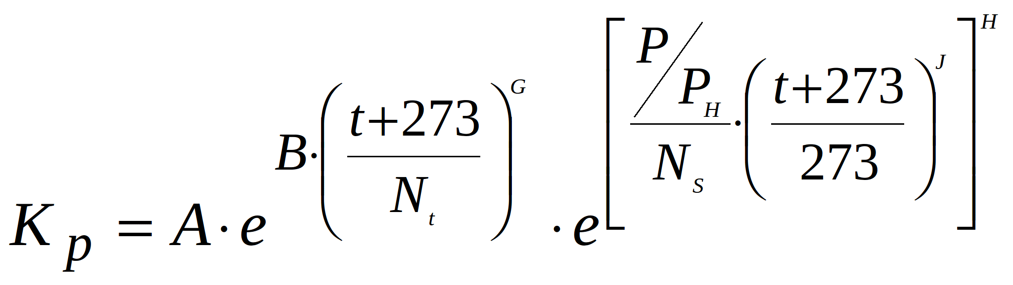
The failure rate for most components can be found using the following mathematical models:

where – initial (basic) failure rate of the component found experimentally by testing it for the non-failure operation, durability, residual life;

– coefficients which modify the initial failure rate depending on various factor(modes and conditions of operation, as well as design, operational, and technological features of the elements);

n – number of factors.

Correction coefficient = k_λ₁k_λ₂k_λ₃k_λ₄ k_λ₅is always greater than one. It indicates that the number of failures can be much greater when the equipment is operated under real-world conditions than when it is operated in a laboratory. Coefficient k_λ₁ represents mechanical factors (vibrations, impact), k_λ₂– environmental factors (temperature, humidity), k_λ₃– operation in low atmospheric pressure, k_λ₄- biological factors, k_λ₅– effects of specific environments. Values of these coefficients can be found in the reference books.

For some complex devices, the total failure rate is the sum of the independent failure rates of the constituent parts of the device (for example, rotating parts and the current coil in a motor). Mathematical model for the failure rate of such a device is given by:

where – initial (basic) failure rate of the j-th constituent part;

m – number of the independent constituent parts;

– correction coefficient of the i-th factor for the j-th part;

– number of factors for the j-th constituent part.

The number of correction coefficients and their mathematical models are defined for a given class of elements. For example, for resistors, the coefficient of the mode of operation is given by:

where: , , , , , , – constants of the model;

t –ambienttemperature °С;

– operating power of the resistor, W;

– nominal power of the resistor, W.

Or, for example, for the integrated circuits, the correction coefficient takes into account the effect of the ionizing radiation. Its value depends on the dose of the ionizing radiation:

dose 0-10 krad, ;

dose 20 krad ;

dose 40 krad .

If the electronics equipment is kept in standby mode (storage) most of the time, with periodicmonitoringof its working condition, then the reliability can be computed with the following models for the failure rates :

For non-moving parts:

For moving parts:

where – failure rate of the element when it is being stored in the original packaging;

– initial (basic) failure rate;

– correction coefficient taking into account ambient temperature;

– coefficient of product acceptance;

– correction coefficient referred to as service factor;

– correction coefficient taking into account the operating conditions in standby mode (storage).

Non-failure operation of an electronic assembly depends on the failure rates of its constituents. The reliability of a non-redundant system with n components in series connection with the independent failure rates of the components (the system remainsoperational,if all components are intact) is:

where - probability of the non-failure operation of the i-th component.

where - failure rate of the system.

The reliability of a redundant system depends on the mode of operation of the duplicate components.

The reliabilities if the systems with passive redundancy and active-active redundancy are described by the same mathematical expressions. If the switch which activates duplicate components is assumed to be instantaneous and completely reliable, then the probability of non-failure operation is

where – reliability of the i-th device; m – number of devices in parallel connection (main + duplicate), – failure rate of the i-th device.

The reliability of the system with active-active redundancy but when the backup components are only lightly loaded (assuming ideal switch) is:

where and – failure rates of the main active device and the i-th backup, respectively.

The reliability of the system with the active-passive redundancy (assuming ideal switch) is:

The reliability of the system with the N+1 redundancy (N active devices and one backup in standby mode) is

where and – failure rates of the active element and the switch, respectively.

The durability of an electronic component depends on the time to fatigue-failure of the component terminals and its residual life. Time to fatigue-failure under harmonic vibrations is given by:

where - number of cycles before failure; f – frequency of vibrations.

The number of cycles to fatigue-failure under harmonic vibrations is given by:

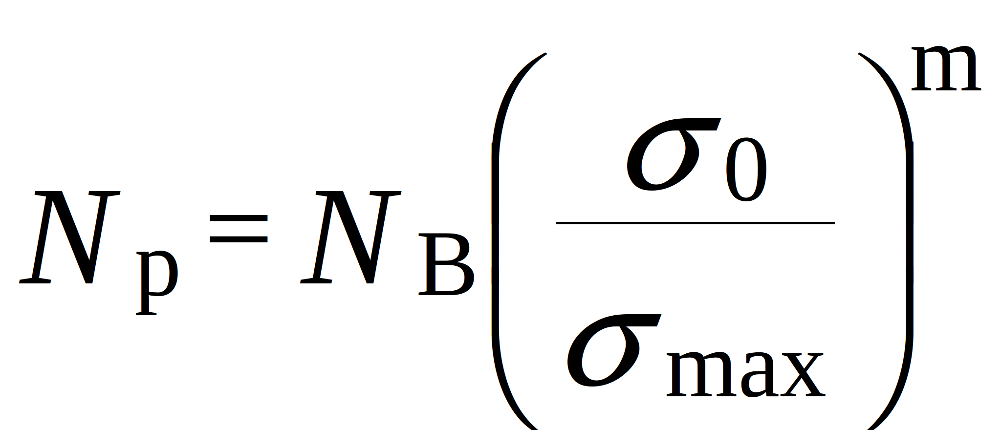
where- fatigue limit; m – parameter which depends on the material, size, and shape of the terminals; - basic number of cycles; - maximum mechanical stress in the terminals.

For the stationary random processes, the hypothesis of the superposition of the fatigue damage under cyclic loading is used. This hypothesis is based on the superposition of the energies of oscillations. Therefore, time to fatigue-failure of the component terminals under random loading can be found

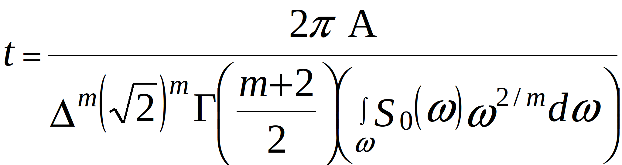
where - standard deviation of stress; - variance; - reduced spectral density; - spectral density; - gamma function; - angular frequency of the harmonic loading ; and - parameters of the fatigue curves where ; - stress amplitude in a cycle; - minimum mechanical stress in the terminals.

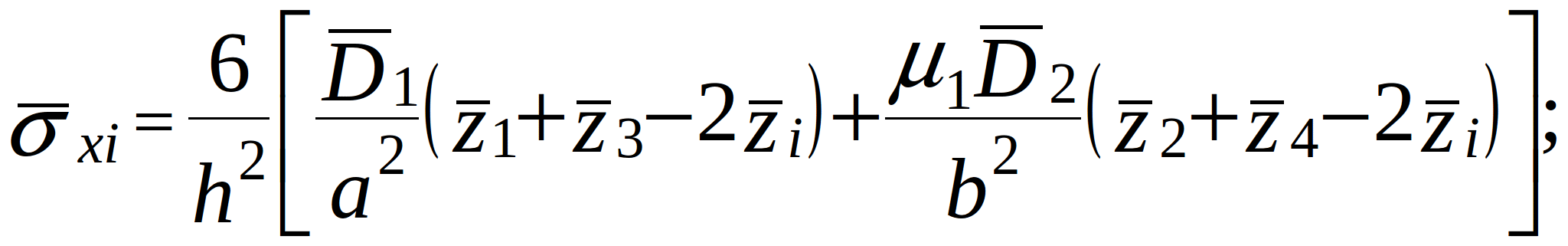
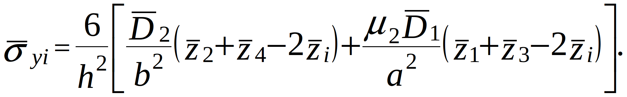
To use the abovementioned formula for the computation of the time to fatigue-failure in the terminals of the components, it is first necessary to compute mechanical stresses in the terminals. Currently, this is done using the Finite Element Method.

Parameterm represents the inclination angle of the fatigue curves. Figure 3.1 shows two experimentally obtained fatigue curves, also known as Wohler curves. They describe the relationship between the stress amplitude and a number of cycles to failure. Curve 1 is for steel of low and medium strength as well as titanium alloys without corrosion and at normal temperature, curve 2 – non-ferrous metals and high-strength alloyed steel. Curve 1 has a sharp bend at cycles, after which it is almost parallel to the abscissa. Therefore, as a basis for tests is usually assumed. Physically, it means that if the stress amplitude is less than , no number of cycles will cause fatigue-failure. This value of stress is called the fatigue limit. Some materials, in particular non-ferrous metals, do not have a distinct fatigue limit: as the number of cycles increases the strength continues to drop (curve 2). For such materials, fatigue is characterized by the finite life threshold (endurance threshold) for a given number of cycles , which is usually taken to be 5*10⁷ cycles. This fully applies to the terminals of electronic components because they are usually made of the non-ferrous metals and their alloys.

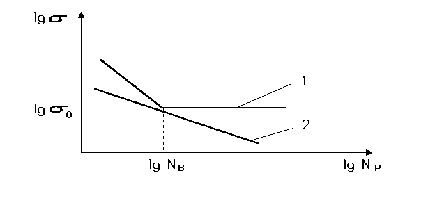
Figure 3.1 Fatigue curves for various materials

Analysis of the thermal modes of electronic assemblies shows that the temperatures at the component terminals do not exceed 150С. Fatiguecurvesfornon-ferrousmetalsand,consequently,parameter , begintochangesignificantlyattemperaturesabove 0,45 - 0,50 T_пл (T_пл – melting point of metal) which, for example, for copper is about 500 С. For othernon-ferrous metalsand alloys, this temperature is either of the sameorder orexceeds it.Thus, theeffect of temperature onthe slope of the fatigue curves for the materials of the terminalscan be neglected. However, temperature plays important role in the mechanical processes occurring in the components. The mechanical effects are transferred to the components through various packaging elements – cabinets, supports, blocks, PCA. Therefore, the effect of temperature on the mechanical processes in the electronic components is accounted for by including the effect of temperature on the supporting structure.

An originalmethod for determiningthe residual lifeof the components was developed. It allows us to take into account the fluctuations inthe electrical characteristics of the circuits, ambient temperature, and the temperatures of the components.

When computing the residual life of an element, the initial data are: structure of the electronics (number of nodes N (blocks etc.), number of components in each node ), failure rates of the elements λj. In this case, the residual life of each electronic component at time is given by